Analysis plans
A central goal of running an experiment is to use data to make decisions that are rigorous and repeatable; an analysis plan is a set of choices and parameters that will govern how Eppo translates the experiment data into dashboards and visualizations–and thus into ship/no-ship decisions.
In general, an experimentation program is most effective if decisions are made in a consistent way across an entire company, and so most of the analysis plan settings can be set on the administration page. However, occasionally you may want to have different settings for certain individual experiments; for example, a website that connects homeowners to contractors is likely to have many more users who are homeowners than contractors, and therefore might use a different statistical approach for an experiment on the contractor on-boarding flow than on the homeowners' search page.
Settings
The experiment-level analysis plan settings are on the experiment setup page.
1. Confidence interval method
Which analysis method to use to estimate the lift and construct the confidence interval.
2. Confidence level
The confidence level represents how often we want the true lift to be inside the confidence interval. The higher the confidence level, the wider the confidence interval needs to be to ensure that it contains the true lift with that level of probability.
A 95% confidence level (the default) means that, for 95% of experiments, the true lift will lie within the respective confidence intervals.1 Lower confidence levels will mean narrower confidence intervals, which in turn means that it is easier to detect a lift as being different from zero (but also more likely that you would incorrectly flag random noise as being a true treatment effect).
3. Multiple testing correction
Use this setting to configure multiple testing correction. When turned on, we ensure that the confidence intervals are widened in order to control for the Family-wise error rate. You can also adjust how much weight to give to the primary metric.
Note, this setting is unavailable for the Bayesian methodology.
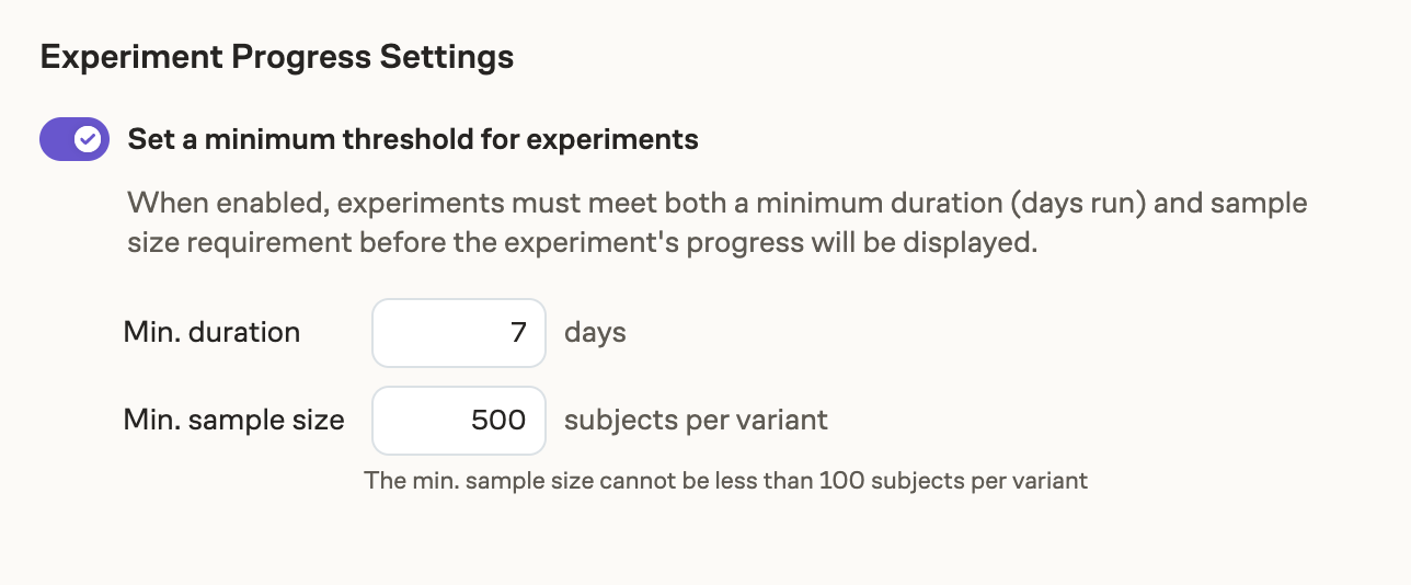
4. Minimum Requirements
If enabled by your admin, these are the minimum run requirements before the progress bar will be displayed. Experiments must meet both the minimum duration (days run) as well as sample size per variant. This is to help prevent premature experiment decisions.
If your admin has not enabled this setting, then minimum requirements will not be visible on experiments.
5. Precision
Precision captures the uncertainty in the point estimate as defined by the width of the confidence interval. Precision is set at the metric level. However, it is possible to override this and set it to a particular value at the experiment level using the analysis plan This is used to power the progress bar, helping you decide when the experiment has run sufficiently long for you to make a decision confidently.
Considerations for setting an analysis plan
You are running an experiment in order to make a decision: should I ship the treatment? Different analysis methodologies might change:
- Which decision you make (and thus whether you make the right decision)
- When you make a decision (which affects development velocity)
- How you make a decision (that is, the decision-making process)
Different methodologies put different constraints on how your team operates day-to-day, and therefore it's important to select one that is compatible with the broader organizational context (such as how velocity is traded off for quality, or any business-determined deadlines or cadences). Perhaps more importantly, though, how experiments are analyzed can dramatically affect how much value you get from running experiments, or even whether you get any value at all.
Here we zoom out to show how the parameters that make up an analysis plan translate to business priorities and constraints, which we hope will help in choosing those parameters.
What's the best way to be wrong?
When picking an analysis methodology, it's important to think about different ways your decision can be wrong:
- False positive (also called Type I error): The treatment has no effect, but you think it does2
- False negative (also called Type II error): The treatment has an effect, but you think it does not
Because you don't know, even after running the experiment, whether the treatment had an effect, you don't know whether observing a nonzero lift is a true positive or a false positive; similarly, not observing a lift could be a true negative or a false negative.
Of course, for any given experiment, you either detect a difference or you don't, and what you want to know is: is this difference (or lack thereof) a true or false positive (or negative)? That is, unfortunately, not possible to know: you can only see the data you've observed, never the underlying process that created the data.
What you can do is (given some assumptions) control the rate of false positives assuming there is no effect, or the rate of false negatives assuming a real effect exists.
In general, statistical significance is about limiting the false positive rate: If your treatment doesn't do anything at all, you want to make sure the random differences between groups are unlikely to be flagged as a significant metric movement.3
Having more statistical power, on the other hand, means that you'll have a lower false negative rate: If there's a real treatment effect, the more power you have the more likely you are to be able to detect a significant metric movement.
Note, though, that these terms don't have the same meaning if using a Bayesian analysis analysis method, although the concepts can still be useful.
Frequentist methods: taking control
The fixed-sample and sequential analysis methods use the framework of null hypothesis significance testing to control the false positive rate: that is, the rate at which a non-effectual treatment would be incorrectly flagged as causing a metric to move. This limits the risk that you will ship treatments based on random noise. Since most treatments don't have much of an effect, this is a useful protection.
These methods do not, however, inherently control the false negative rate: the rate at which a treatment with a real effect will go undetected; that requires ensuring that you have enough data (and therefore enough power) to detect any treatment effect that actually exists. (Using Eppo's Sample Size Calculator is a great way to do that.)
The biggest difference between these methods is in how flexible they are, given the guarantees: fixed-sample analysis can detect a lift more quickly, but you only have one shot to look at the results and make a decision, while sequential analysis is more forgiving and allows you to continuously check the results and make a decision at any point.
Bayesian methods: telling you what you actually want to know
Bayesian methods, in contrast, make no guarantees about either false positive or false negative rates. Instead, the goal is to provide a description of your beliefs about what the true lift is (meaning, how likely is any particular lift, not just whether the lift is zero or nonzero).
Before you run the experiment, you have some prior beliefs about the treatment (that is, your best guess of what the lift will be, as well as your level of certainty about that guess). Once you run the experiment, you use the data you observe to update your prior beliefs, resulting in a posterior distribution that describes how likely you believe different lifts to be.
Although it can be disconcerting not to have the "guarantees" provided by frequentist methods, a Bayesian would argue that those guarantees don't actually guarantee anything useful: they can tell you how likely a true lift will be missed or a nonexistent lift will be falsely detected, but not how likely a lift (or lack thereof) is to be true. Bayesian methods can tell you this–as long as you trust your prior and your assumptions about the structure of the data.
And, importantly, while frequentist methods provide a binary structure for making decisions—an effect exists or does not—Bayesian methods allow for a more nuanced way of making decisions, which in particular is useful when sample sizes are too small to be able to detect even reasonable lifts with a frequentist method. Bayesian methods also allow you to make decisions at any time, and make it easier to tailor the level of rigor to the potential costs of being wrong: you can move fast when being wrong is cheap, and be more thorough when it is expensive.
Being the right amount of wrong
Setting the confidence level determines how easy it is to flag a difference in a metric as "significant"; thus—regardless of the analysis method—a lower confidence level means you will be more likely to treat random noise as if it were a real treatment effect. It will also mean, however, that a real treatment effect will be detected more quickly.
Collecting more data will—regardless of the analysis method—mean that you will be less likely to miss a real treatment effect. It also means, though, that you will have to wait longer to recognize when there is no treatment effect—you'll make decisions more slowly.
The goal for picking an analysis plan is to balance:
- How often you will be wrong in each direction (false positive or false negative)
- The costs of being wrong in each direction (would you rather miss a true effect, or ship a dud?)
- How long it will take to make a decision
- How easy it will be to make a decision (including how easy it is to communicate about and align on a decision)
Footnotes
-
For anyone used to thinking in p-values, this corresponds to a p-value of 0.05 (that is, ) ↩
-
"Positive" here means effect detected, and "negative" means no effect detected; think of a diagnostic test for a disease, where "positive" means that the disease is present, and "negative" means it is not. In particular, a "positive" result in this sense would be observing a difference, in either direction, between treatment and control. That is, having a confidence interval that is entirely above or below zero would be considered a "positive" result in the sense of false (or true) positive (or negative. ↩
-
Specifically, if your confidence level is set to 95%, then a statistically significant result should happen no more than 5% (i.e. 1 - 95%) of the time in an A/A test that compares different groups receiving identical experiences. ↩